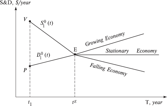
By analogy with classical mechanics, we can treat these prices and quantity functions as the trajectories of movement of the market agents in the two-dimensional economic PQ-space as it was displayed in Fig. 3.

In principle, this representation gives nothing new in comparison with Figs. 1 and 2. Nevertheless, there is one interesting nuance here, in which the similarity of this diagram can be compared to the traditional picture in the conceptual neoclassical model of S&D. We will examine this question below. But let us now focus attention on the following nuances in the picture in Fig. 3. First, it is clearly shown by the arrows, that the buyer and the seller seemingly move towards each other on the price, with the seller reducing it, and the buyer, on the contrary, increasing it. From this, we can reflect on the illustration of normal market negotiation processes. Secondly, usually the quotations of quantities are reduced during the process of negotiations both by the buyer and by the seller. Clearly, all agents want to purchase or to sell a smaller quantity of goods at the compromise market price than at the most desired, presented at the very beginning of trading.

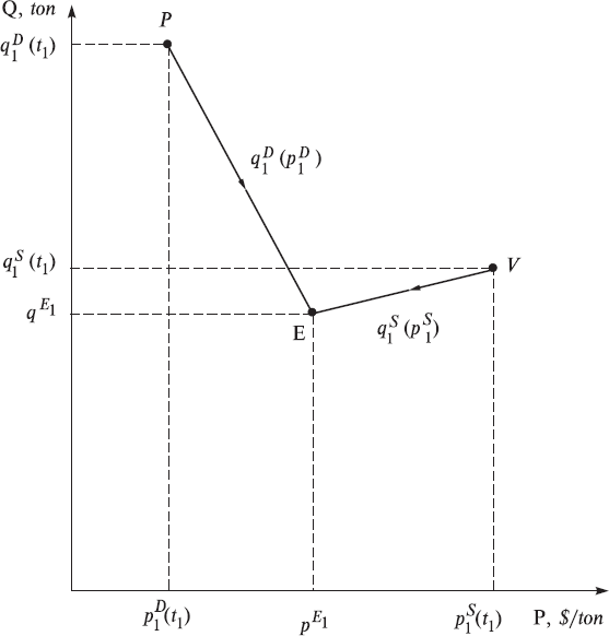
Fig. 3. Dynamics of the classical two-agent market economy in the two-dimensional economic price-quantity space within the first time interval [t₁, t₁^E].

And now we turn from the simplest economy to a more developed economy, in which the farmer and hunter gradually switch from the discrete trade system (one trade per year) to the continuous trade system on the market. Generally speaking, negotiations are conducted continuously and transactions are accomplished continuously, depending on the needs of the buyer and the seller. This would continue for many years. Taking into account this new long-term outlook it is expedient to change somewhat the method of describing the work of the market. Namely, by quotations of a quantity of goods, it is now more convenient to represent a quantity of goods during a specific and reasonable period of time, for example year, if the discussion deals with the long-standing work of the market. In this case the dimension of a quantity would be represented by ton/year. We show in Figs. 4, 5 how it is possible to graphically represent the work of the market over a long span of time. We see that before the establishment of equilibrium at point E, transactions were of course accomplished, but probably did not bring maximum satisfaction to the participants in the market. This would induce agents to continue to search for long-term compromises in prices and quantities. After reaching equilibrium, the volume of trade reaches a maximum, and participants in the market therefore attempt to further support this equilibrium.

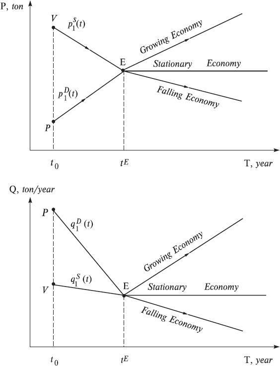
Fig. 4. The classical stationary and non-stationary two-agent market economies in the [T, P] and [T, Q] coordinate systems in the time interval t > t^E.

Fig. 5. The classical stationary and non-stationary two-agent market economies in the [T, S&D] – coordinate system.

Here a fork appears in the following theory: – look at Figs. 5 and 6. If quotations cease to change, then the economy converts to a stationary state in which time appears to disappear. This is especially noticeable in Fig. 6, where this sort of stationary state is described by one point, E. We will label the economies in the stationary state simply the stationary economies. But if quotations vary with time, then the economy will be named the time-dependent or simply non-stationary economies. In Figs. 5 and 6 they are represented by two lines, which emanate from the equilibrium point E. If in this case the equilibrium quantity grows, then the economy is a growing one. But if it decreases, then the economy is falling one, which clearly is represented in Fig. 5. As a rule, in such cases, the total S&D behave similarly and this can be easily seen in Fig. 5. Let us note that their dimensions in this model have also changed, now equaling $ · ton/year.

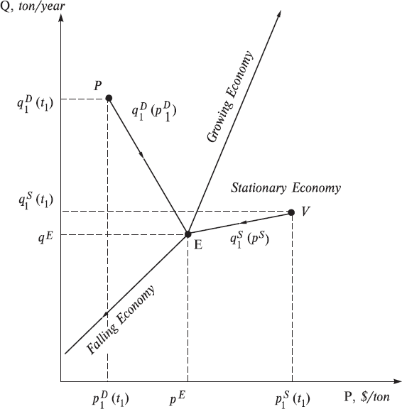
Fig. 6. The classical stationary and non-stationary two-agent market economies in the economic price-quantity space at t > t^E.

Now we will increase the level of complexity of the classical economies by examining how it is possible to incorporate several buyers and sellers into the theory. It is understandable that each market agent will have its own trajectories in the PQ-space. In principle, they can vary greatly. There is good reason to believe that there is much similarity in the behavior of all buyers in general. The same is valid of course for all sellers. The reason is as follows. There is the intense information exchange on the market, by means of which the coordination of actions is achieved among the buyers, among the sellers, as well as among the buyers and sellers. This coordination is carried out to assist the market in reaching its maximum volume of trade, since it is precisely during the process of trading that the last point is placed in the long process of preliminary business operations: production, financing, logistics, etc. This is exactly what we would have referred to earlier as the social cooperation of the market’s agents. For example, it is natural to expect that all buyers, from one side, and sellers, from other side, behave on the market in approximately the same way, since they all are guided in their behavior on the market by one and the same main rule of work on the market: “Sell all – Buy at all”.

Hence it is possible to draw from the above discussion the following important conclusion: the trajectories of all buyers in the P-space will be close to each other; therefore, the totality of all buyers’ trajectories can be graphically represented in the form of a relatively narrow “pipe”, in which will be plotted the trajectories of all buyers. It is also possible to represent all price trajectories of the buyers by means of a single averaged trajectory, p^D(t), which we will do below. We will do the same for the sellers, and their single averaged price trajectory we will designate as p^S(t).

We have a completely different situation with the quantity trajectories, since each market agent can have the very different quantities, bearing in mind the fact that the behavior of the buyers’ (sellers’) curves can be relatively similar to each other. Nevertheless, we can establish some regularities in the behavior of the whole market, being guided by common sense and the logical method. Since the quotations of quantities are real in the classical models, we can add them in order to obtain the quantity quotations of the whole market, q^D(t) и q^S(t). However one should do this separately for the buyers and sellers as follows:

where summing up of quantity quotations is executed formally for the market, which consists of N buyers and M sellers. In this case we understand that for the whole market we can draw all the same pictures as displayed in Figs. 1–6 for the two-agent market. Thus, for instance, we can represent the dynamics of our many-agent market by the help of the following pictures in Fig. 7. In it, the dynamics of many-agent market are depicted at the moment of equilibrium (curves q^D(p^D) and q^S(p^S)), as well as dynamics of the stationary economy (point E) and dynamics of the non-stationary growing and falling economies.