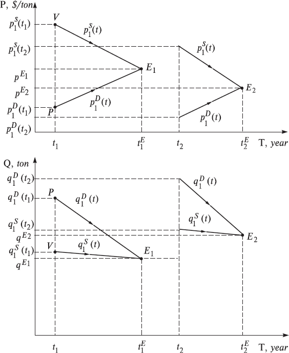
Fig. 1. Trajectory diagram displaying dynamics of the classical two-agent market economy in the one-dimensional economic price space (above) and in the economic quantity space (below). Dimension of time t is year, dimension of the price independent variable P is $/ton, and dimension of the quantity independent variable Q is ton.
A voluntary transaction is accomplished to the mutual satisfaction. Further, the market again is immersed into the state of rest until the next harvest and its display to sale next year at the moment in time of t2. Harvest in this season grew, therefore q1S(t2)> q1S(t1). In this situation, the seller is, obviously, forced to immediately set out the lower starting price, p1S(t2)< p1S(t1), while the buyer, seizing the opportunity, also reduced their price and increased their quantity of grain: p1D(t2)< p1D(t1) and q1D(t2)> q1D(t1). It is natural to expect in this case that the trajectories of the buyer and the seller would be slightly changed, and agreement between the buyer and the seller will be achieved with other parameters than in the previous round of trading.
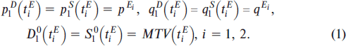
Conventionally, we will describe the state of the market at every moment in time by the set of real market prices and quantities of real deals which really take place in the market. As we can see from the Fig. 1 real deals occur in the market in our case only at the moments t1E and t2E when the following market equilibrium conditions are valid (points Ei in Fig. 1):
In this formula, we used several new notions and definitions, whose meanings need explanation. Let us make these explanations in sufficient detail in view of their importance for understanding the following presentation of physical economics. First, in contemporary economic theory, the concept of supply and demand (S&D below) plays one of the central roles. Intuitively, at the qualitative descriptive level, all economists comprehend what this concept means. Complexities and readings appear only in practice with the attempts to give a mathematical treatment to these notions and to develop an adequate method of their calculation and measurement. For this purpose, the various theories contain different mathematical models of S&D that have been developed within the framework. In these theories, differing so-called S&D functions are used to formally define and quantitatively describe S&D.
In this book, we will also repeatedly encounter the various mathematical representations of this concept in different theories, which compose physical economics, namely, classical economy, probability economics, and quantum economy.
Even within the framework of one theory, it is possible to give several formal definitions of S&D functions supplementing each other. For example, within the framework of our two-agent classical economy, we can define total S&D functions as follows:

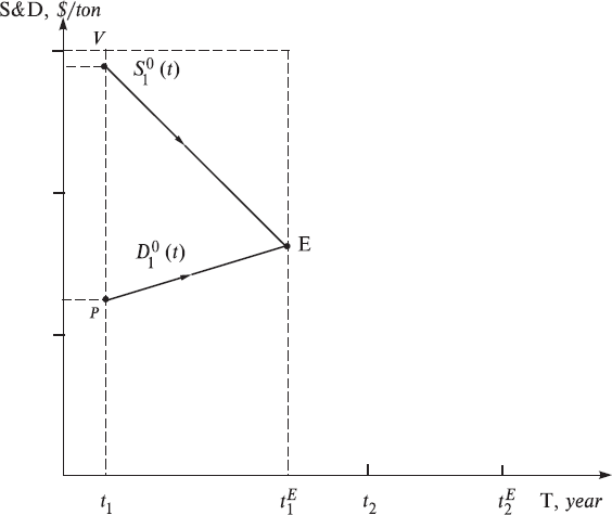
Thus, we have defined at each moment of time t the total demand function of the buyer, D10(t), and the total supply function of the seller, S10(t), as the product of their price and quantity quotations. These functions can be easily depicted in the coordinate system of time and S&D [T, S&D], as it was done in Fig. 2 displaying the so-called S&D diagram. As one would expect, the S&D functions intersect at the equilibrium point E. It is accepted in such cases to indicate that S&D are equal at the equilibrium point. We consider that it is more strictly to say that equilibrium point is that point on the diagram of the trajectories, where these trajectories intersect, i.e., where the price and quantity quotations of the buyer and the seller are equal. But that in this case S&D curves intersect is the simple consequence of their definition equality of prices and quantities at the equilibrium point.
The last observation here concerns a formula for evaluating the volume of trade in the market, MTV(tiE), between the buyer and the seller where they come to a mutual understanding and accomplishment of transaction at the equilibrium point Ei. It is clear that to obtain the trade volume (total value of all the transactions in this case), it is possible to simply multiply the equilibrium values of price and quantity that are derived from the above formula. The dimension of the trade volume is of course a product of the dimensions of price and quantity; in this example this is $. The same is valid for the dimensions of the total S&D, D10(t) and S10(t).
Fig. 2. S&D diagram displaying dynamics of the classical two-agent market economy in the time-S&D functions coordinate system [T, S&D], within the first time interval [t1, t1E].
4.2. The Main Market Rule “Sell all – Buy at all”
Having a method to more or less evaluate the price quantitatively is always advantageous, as it helps us to somewhat predict market prices. Using the main rule of work on the market is used to this end, and this strategic rule of decision making can be briefly formulated as follows: “Sell all – Buy at all”. This main market rule indicates the following different strategies of market actions (action on the market is setting out quotations) for both the seller and the buyer. For the seller this strategy consists in striving to sell all the goods planned to sale at the maximally possible highest prices. Whereas for the buyer this strategy consists in the fact that it will expend all the money planned for the purchase of goods and try to purchase in this case as much as possible at the possible smallest price. Thus, the main market rule leads to the corresponding algorithms of the actions of agents on the markets, which are graphically represented in the form of agents’ trajectories in the pictures. The point of intersection and the respective trade volume in the market, MTV, are easily found with the help of the following mathematical formulas:
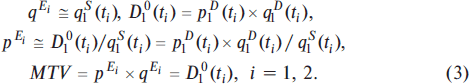
It is natural here to name D10(t1) the total demand of buyer at the initial moment of trading. The sense of this quantity is in the fact that this is quantity of resources, planned for the purchase of goods, expressed in the money, although the dimension of this demand is the dimension of money price ($/ton) multiplied by the dimension of quantity (ton). In our case, this is $. We emphasize that, over the course of development of quantitative theory, this is very important in order to draw attention to the dimension of the used quantities and parameters, and to the normalization of the applied functions (see below).