Formulas for demand have a similar structure naturally:

To avoid misunderstandings, note that formulas (1.17) and (1.21) express the relationship known for Gaussians between their agent frequency parameters and the widths, more precisely, the widths of Gaussians at half-height. The numerical values of these widths are set or selected explicitly or implicitly by the agents themselves, just as prices and quantities are set by them. But, very importantly, unlike price and quantity quotations, the «quotations» of widths are not explicitly exhibited either in negotiations or in organized markets. The values of these widths may not even be accurately realized by the agents themselves; in this respect, agents may act purely intuitively, depending on the market situation.

Summing up the intermediate results, we can briefly say that in this version of the theory the buyer's probabilistic demand function is described by four parameters, the price p^D, the quantity q^D and two widths Г^DР and Г^DР. The same statement is of course true for the seller's probabilistic supply function. It is these eight parameters that take into account all of the relevant market information that the buyer and seller use before they put up quotations at any given time in the process of trading in the market. And let us emphasize for clarity that usually both buyers and sellers declare or announce publicly and unambiguously only their price and quantity quotations, leaving the information about their widths "behind the scenes".

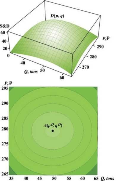
For our model grain market the probability functions S&D are presented graphically in Figs. 1.6–1.9.

Obviously, for a two-agent economy, all S&D market function surfaces have a simple smooth structure with one maximum. Of course, for more complex economies the structure of the surfaces will be much more complex.

Fig. 1.6. Graphical representation in the rectangular two-dimensional coordinate system [P, S& D] of one-dimensional price functions d^P (p) and s^P (p) as two-dimensional curves with maxima at prices p^D and p^S and widths Г^DР and Г^SР respectively. The values used for the widths are: Г^DР = 23.8 $/ton, Г^SР = 37.0 $/ton.

Fig. 1.7. Graphical representation in the rectangular two-dimensional coordinate system [P, S& D] of one-dimensional quantity functions d^Q(q) and s^Q(q) as two-dimensional curves with maxima at quantities q^D and q^S and widths Г^DQ and Г^SQ respectively. The values used for the widths are: Г^DQ = 26.4 ton / year, Г^SQ = 6.8 ton/year.

Below we will discuss in detail all new concepts, main features and calculation details for our simplest two-agent system, so that we will not be distracted by their discussion in further consideration of more complex issues concerning the exchange. So, by definition and in its essence, the probabilistic function of demand D(p,q) (supply S(p,q)) is the probability of the buyer (seller) concluding a deal to buy and sell the traded goods in quantity q at price p. If this is so, then, according to the standard concepts of probability theory, it is natural to define the probability of the transaction under these conditions as the multiplication of these probabilities:

We call this probability of making a deal a market deal function, and, for convenience, we also refer it to the market functions of supply and demand. Like the market functions D(p, q) and S(p, q), it is dimensionless. For the sake of certainty, let us explain that, generally speaking, purchase and sale transactions can occur in the market at any time, at any price and in any quantity, within reasonable limits, but with varying degrees of probability. But if the transaction function is a sufficiently high and narrow bell with a single maximum with the parameters p^M and q^M, then almost all transactions will occur in the proximity of these values, so it is reasonable to consider these very values to be market prices and quantities. If the function of transactions looks otherwise, of course, these definitions are somewhat meaningless, and one should consider the mechanism of probabilistic pricing in detail. Below we will always assume that the function of transactions is such as to allow market prices and quantities to be determined in a fairly simple way. This is exactly the case we have graphically presented in Fig. 1.10 for our two-agent model of the grain market.

Fig. 1.8. Graphical representation in a rectangular three-dimensional coordinate system [P, Q, S&D] of the two-dimensional buyer demand function as a three-dimensional surface D (p, q) with a maximum at the point A (p^D, q^D) in the plane (P, Q).

Fig. 1.9. Graphical representation in the rectangular three-dimensional coordinate system [P, Q, S&D] of the two-dimensional seller's supply function as a three-dimensional surface S(p, q) with a maximum at point B (p^S, q^S) in the plane (P, Q).

As expected, the surface of the market transaction function F(p, q) has only one maximum. For multi-agent economies, the structure can be much more complex.

Fig. 1.10. Three-dimensional graphical representation in a rectangular three-dimensional coordinate system [P, Q, F] of the three-dimensional deal surface F(p, q) in the form of a high and narrow bell with one maximum at the point C (p^M, q^M) in the plane (P, Q). The graphical method of calculation gives the following results for market prices and quantities: p^M = 281.4 $/ton, q^M = 51.9 ton/year.

Let us now turn to the question of calculating market prices and quantities within the framework of probabilistic economics. It is well known from the standard course of mathematical analysis that extrema of a multidimensional function should be defined as points on the corresponding surface in which the total differential of this function is 0. In our situation this condition leads to the following equation: